Data Transformation ToolsTypes of Data Transformation: Best Practices and Examples
Multi-chapter guide | Chapter 4
One article can’t contain all types of data transformation because they are practically limitless. For this article, we picked a few that belong in the modern toolbox of every data engineer, broadly grouped into two categories:
Structural transformations (data harmonization, data normalization and denormalization, and destructive transformation)
Attribute-level transformations (data watermarking, data obfuscation, and data imputation)
Structural data transformations involve changes to a data table structure or relationships (e.g., altering schema or data model). In contrast, attribute-level transformations focus on modifying individual data attributes or fields (e.g., encoding data or replacing missing data with estimated values).
As the number of data pipelines grows, following best practices to implement transformations has far-reaching implications. The chosen implementation method impacts how easy it would be to troubleshoot a latency problem, update the code after a schema update, pass a regulatory audit or scale the application environment without overrunning the infrastructure budget.
This article explains several types of data transformations, their purposes, and some implementation best practices, all while providing hands-on examples using Scala 3.
For readers not comfortable with mastering a programming language to transform data, the last section of this article introduces the leading open-source project that allows data engineers to implement transformations using declarative YAML files. As we will explain, this approach has multiple benefits beyond lowering the required programming skill level.
Summary of types of data transformation
| Structural Transformations | |
|---|---|
| Data harmonization | This type of transformation aims to align data from different sources to a common format and standard. |
| Data normalization and denormalization | This method reduces data redundancy, improves data usability and integrity, or improves performance. |
| Data normalization of hierarchical structures | This type of transformation anonymizes sensitive data into an unreadable format. |
| Destructive transformation | Such transformations delete obsolete or irrelevant aspects of the data, reduce bloat, and improve performance. |
| Attribute-Level Transformations | |
| Data aggregation and pre-calculation | This approach involves embedding invisible markers within data to track and protect its integrity. |
| Data imputation | Imputation involves filling in missing data entries with estimated or calculated values. |
| Combining Transformations | |
| Data waterfall or pipeline | This practice involves sequentially applying multiple transformations where each step builds on the previous one. |
Below is a summary of the contents we will review during this article:
Overview of types of data transformation
The next sections of the article explain the transformations using examples in Scala 3 in the same order presented in the above summary table.
Structural transformations
As their name suggests, structural transformations deal with changes directly related to the dataset's structure. Hence, the most common operations involved in this process might include rearranging, combining, and renaming data structures.
Structural transformations improve data categorization, organization, and access. They make data more intuitive and accessible for users and improve the efficiency of data retrieval and analysis processes in customer relationship management systems.
Data harmonization
This technique involves aligning data from different sources to a common format and standard. This can include standardizing attributes such as date formats, units of measure, and terminology.
Data harmonization can use pure functions to standardize data formats.
Consider an example of a data source containing dates in different formats. The objective is to harmonize the formats to have a uniform date structure.
We can define a simple function that will unify formats:

import java.time.LocalDate
import java.time.format.DateTimeFormatter

// Function to harmonize date format to "yyyy-MM-dd"
def harmonizeDate(dateStr: String, inputFormat: String): String = {
  val inputFormatter = DateTimeFormatter.ofPattern(inputFormat)
  val outputFormatter = DateTimeFormatter.ofPattern("yyyy-MM-dd")
  val date = LocalDate.parse(dateStr, inputFormatter)
  date.format(outputFormatter)
}

// Example usage
val dates = List(
  ("01-31-2024", "MM-dd-yyyy"), // Data source 1
  ("31/01/2024", "dd/MM/yyyy"), // Data source 2
  ("2024/01/31", "yyyy/MM/dd") // Data source 3
)

val harmonizedDates = dates.map { case (dateStr, format) => harmonizeDate(dateStr, format) }

// Output the harmonized dates
harmonizedDates.foreach(println)
This will result in the following:
// 2024-01-31
// 2024-01-31
// 2024-01-31
Data normalization
It involves structuring data based on normalization rules to reduce data redundancy, improve data usability and integrity, or improve performance, especially when re-organizing data from multiple systems into a combined data model. This technique decomposes a central data structure into several structures using attributes as breaking points. Developers often adopt the Third Normal Form (3NF) schema design approach, which ensures that non-key attributes directly depend on the primary key, eliminating transitive dependencies. The result is a system of data structures related to each other via keys.
A modern example of this philosophy is the Inmon Method, also called Bill Inmon, or the Inmon Approach; it focuses on building a “single source of truth,” thereby opening possibilities for complex reporting and analysis.
However, while this method can be advantageous for storage optimization, it shouldn’t always be practiced because it might increase query complexity, involve high storage requirements, and cause computational overhead resulting from more JOIN operations. Modern platforms like DataForge allow developers to model data in a 3NF schema design without the usual storage and performance overhead.
Below we discuss an example where we normalize a JSON hierarchical structure to a 3NF (third normal form).
It is common in modern applications to find nested data structures in formats such as JSON, particularly if we’re dealing with data from APIs. These structures are highly flexible, but can be challenging to query efficiently, especially as the nesting level increases.
Data normalization of hierarchical structures can help us flatten these structures into a more manageable format, improving both performance and ease of manipulation.
Let us think of an example where we have an e-commerce website that handles customer orders using nested JSON data structures; we would like to traverse the nested structure and flatten it for further processing.
For this example, we’ll need a reliable Scala 3 JSON parsing library. We’ll use circe since it’s well-maintained and offers robust type safety. However, there are many other third-party alternatives.
Once we have our circe dependency properly defined in our build file, we can import the required modules and define our sample dataset:
Data normalization of hierarchical structures
import $ivy.`io.circe::circe-core:0.14.5`
import $ivy.`io.circe::circe-parser:0.14.5`

import io.circe._, io.circe.parser._

val jsonString = """
{
  "orderId": "12345",
  "customer": {
	"id": "C789",
	"name": "Alice Johnson",
	"address": {
  	"street": "123 Main St",
  	"city": "Techville",
  	"zipcode": "98765"
	}
  },
  "items": [
	{
  	"productId": "P111",
  	"name": "Laptop",
  	"price": 999.99,
  	"quantity": 1
	},
	{
  	"productId": "P222",
  	"name": "Mouse",
  	"price": 24.99,
  	"quantity": 2
	}
  ],
  "totalAmount": 1049.97
}
"""
Next, we define our flattening function. This method will recursively traverse the nested JSON structure, creating a flap map where nested objects are represented with dot notation in the keys:
def flattenJson(json: Json, prefix: String = ""): Map[String, String] = json.fold(
  jsonNull = Map(prefix.init -> "null"),
  jsonBoolean = b => Map(prefix.init -> b.toString),
  jsonNumber = n => Map(prefix.init -> n.toString),
  jsonString = s => Map(prefix.init -> s),
  jsonArray = arr => arr.zipWithIndex.flatMap { case (j, i) =>flattenJson(j, s"$prefix$i.") }.toMap,
  jsonObject = obj => obj.toList.flatMap { case (k, j) => flattenJson(j, s"$prefix$k.") }.toMap
)
As we can see, we’re taking care of multiple possible nested data structures; null, boolean, number, and string values are handled by creating simple key-value pairs, while other structures such as arrays and objects are recursively flattened.
Finally, we can parse our original data structure and apply our flattening method:
val result = parse(jsonString) match {
  case Right(json) => flattenJson(json)
  case Left(error) => Map("error" -> error.toString)
}

result.foreach { case (k, v) => println(s"$k: $v") }
In the end, we get a flat structure that is easily transferable to virtually any conventional structure (e.g., a tabular structure):
// items.1.name: Mouse
// items.1.quantity: 2
// orderId: 12345
// items.0.productId: P111
// customer.id: C789
// totalAmount: 1049.97
// items.1.productId: P222
// customer.address.street: 123 Main St
// items.0.name: Laptop
// items.0.price: 999.99
// items.1.price: 24.99
// customer.address.zipcode: 98765
// items.0.quantity: 1
// customer.address.city: Techville
// customer.name: Alice Johnson
import $ivy.`io.circe::circe-core:0.14.5`
import $ivy.`io.circe::circe-parser:0.14.5`
// Note: We need to import generic derivation, and automatically derive decoders setting auto flag below
import $ivy.`io.circe::circe-generic:0.14.5`
import io.circe._, io.circe.parser._
// Automatically derive decoders
import io.circe.generic.auto._
import $ivy.`io.circe::circe-parser:0.14.5`
// Note: We need to import generic derivation, and automatically derive decoders setting auto flag below
import $ivy.`io.circe::circe-generic:0.14.5`
import io.circe._, io.circe.parser._
// Automatically derive decoders
import io.circe.generic.auto._
Next, we can define our input and output classes. These will be the base for how we represent our sample JSON data structure as well as the resulting schema:
// Define input Classes
case class OrderJson(orderId: String, customer: Customer, items: List[Item], totalAmount: BigDecimal)
case class Customer(id: String, name: String, address: Address)
case class Address(street: String, city: String, zipcode: String)
case class Item(productId: String, name: String, price: BigDecimal, quantity: Int)

// Define output Classes
case class OrderNoNesting(orderId: String, customerId: String, totalAmount: BigDecimal)
case class ItemsWithOrderId(orderId: String, productId: String, name: String, price: BigDecimal, quantity: Int)
Next, we declare our simple example JSON data structure:
val jsonString = """
val jsonString = """
{
  "orderId": "12345",
  "customer": {
	"id": "C789",
	"name": "Alice Johnson",
	"address": {
  	"street": "123 Main St",
  	"city": "Techville",
  	"zipcode": "98765"
	}
  },
  "items": [
	{
  	"productId": "P111",
  	"name": "Laptop",
  	"price": 999.99,
  	"quantity": 1
	},
	{
  	"productId": "P222",
  	"name": "Mouse",
  	"price": 24.99,
  	"quantity": 2
	}
  ],
  "totalAmount": 1049.97
}
"""
Finally, we define our parsing and normalization function, and apply the transformation to our original data structure:
// Function to parse JSON and normalize into 3NF
// Function to parse JSON and normalize into 3NF
def normalizeOrder(jsonStr: String): Either[Error, (OrderNoNesting, List[ItemsWithOrderId], Customer, Address)] = {
  decode[OrderJson](jsonStr).map { order =>
	val orderNoNesting = OrderNoNesting(order.orderId, order.customer.id, order.totalAmount)
	val itemsWithOrderId = order.items.map(item =>
  	ItemsWithOrderId(order.orderId, item.productId, item.name, item.price, item.quantity)
	)
	(orderNoNesting, itemsWithOrderId, order.customer, order.customer.address)
  }
}

// Usage
normalizeOrder(jsonString) match {
  case Right((order, items, customer, address)) =>
	println("Normalized Order:")
	println(s"Order: $order")
	println("Items:")
	items.foreach(println)
	println(s"Customer: $customer")
	println(s"Address: $address")
  case Left(error) =>
	println(s"Error: $error")
}
The result is a normalized version of the original JSON nested structure, which effectively flattens the hierarchical data into separate, related entities:
// Normalized Order:
// Order: OrderNoNesting(12345,C789,1049.97)
// Items:
// ItemsWithOrderId(12345,P111,Laptop,999.99,1)
// ItemsWithOrderId(12345,P222,Mouse,24.99,2)
// Customer: Customer(C789,Alice Johnson,Address(123 Main St,Techville,98765))
// Address: Address(123 Main St,Techville,98765)
Data denormalization
Denormalization involves adding redundant data to one or more data structures to make JOIN operations in relational databases more cost-effective. While it might initially seem that normalization and denormalization are mutually exclusive, that is not the case; both techniques can be used simultaneously, depending on the environment and ultimate goals.
For example, we might encounter a system using a set of core structures with low tolerance for data inconsistencies, low access, and high demand for integrity. This system might also involve another set of read-heavy structures that require the most optimal query performance. In such a scenario, we would use a normalized approach for the core entities and a denormalized approach for the read-heavy components.
Let us think of an example where we have a MOOC (Massive Open Online Course) platform offering various courses to students:
| Table | Attributes |
|---|---|
| Courses |
|
| Instructors |
|
| Categories |
|
| Students |
|
We can think of this system as normalized:
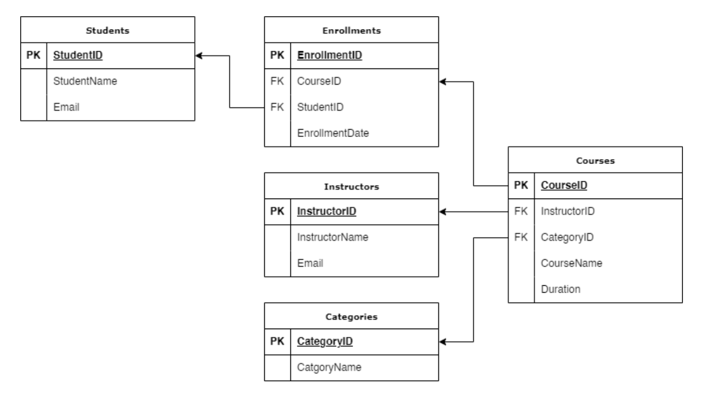
Figure 1: Database Schema in 3NF
Where we have one table for each entity.
We can also think of it using a hybrid approach:

Figure 2: With Denormalized Table
Lastly, we can rebuild our system to be completely denormalized (i.e., a single table):

Figure 3: A Completely Denormalized Architecture
Ultimately, the choice between normalized and denormalized data structures depends on the number of data sources and tables, performance requirements, and the data architect’s preferences. Normalized structures are optimized for write operations and help maintain data integrity by avoiding duplication. On the other hand, denormalized structures are optimized for read performance by reducing the need for complex joins, which can improve query speed but at the cost of potential data inconsistencies.
The proliferation of modern columnar file formats like Parquet has shifted the balance. These formats offer efficient compression and reduced storage costs, even with duplicated data elements within a column, making denormalized structures more practical and less costly. As a result, denormalization has become more common, particularly in analytics workloads where read performance is critical.
Destructive transformation
Consists of intentionally deleting obsolete or irrelevant aspects of the data to reduce bloat and improve performance. It can use immutable data structures where transformations produce new datasets with obsolete data removed. It frees up storage space and improves query performance by removing outdated data, ensuring the database remains efficient and focused on current inventory.
Let us consider an example of managing office supplies using a simple database schema. We have had three transactions in a week and would like to remove unnecessary information using functional methods.
We first declare our simple transformation function:
// Perform destructive transformation and print the results in a single pass
def anonymizeDescriptions(transactions: List[(Int, Double, String)]): List[(Int, Double, String)] = {
  transactions.map { case (id, amount, _) =>
    (id, amount, "REDACTED")
  }
}
Next, we define our target data structure:
// Original data structure
val transactions: List[(Int, Double, String)] = List(
  (101, 250.0, "Payment for office supplies"),
  (102, 320.5, "Payment for software subscription"),
  (103, 150.75, "Refund from hardware return")
)
Finally, we transform our original data structure:
// Output the transformed data
val transformedTransactions = anonymizeDescriptions(transactions)

// Assign output data to a new variable for further processing
val outputData: List[(Int, Double, String)] = transformedTransactions
Resulting in the following:
outputData: List[Tuple3[Int, Double, String]] = List(
  (101, 250.0, "REDACTED"),
  (102, 320.5, "REDACTED"),
  (103, 150.75, "REDACTED")
)
Here, we are using single-pass processing, which minimizes the number of data traversals. This is especially useful when transforming large data structures.
Attribute-level transformations
Attribute-level transformations modify individual data attributes within a dataset rather than changing its structure or schema.
These transformations may involve enrichment processes such as data imputation for missing values, protection mechanisms such as watermarking and obfuscation, and data standardization via mathematical or statistical techniques.
In the next section, we will discuss three core data transformation techniques.
Data aggregation and pre-calculation
Data aggregation and pre-calculation involve computing summary statistics from existing data attributes. This method can improve query performance and simplify posterior data transformations & analysis by storing a form of precomputed values as a new column, along the original data structure.
Let us present a situation where we would like to perform an aggregation operation on a dataset containing sales data for an electronics shop. We’ll calculate the total sales value for each product and add it as a new field to our data structure.
We can start by defining our input and output data structures:
// Input data structure
case class SalesRecord(id: Int, product: String, amounts: List[Double])

// Output data structure
case class SalesRecordResult(id: Int, product: String, amounts: List[Double], total: Double)
Next, we can create sample data entries by creating SalesRecord instances using the `SalesRecord` class:
// Sample data
val salesData = List(
  SalesRecord(1, "Laptop", List(999.99, 1299.99, 1499.99)),
  SalesRecord(2, "Mouse", List(19.99, 24.99, 29.99)),
  SalesRecord(3, "Keyboard", List(49.99, 69.99, 89.99))
)
Finally, we can perform our transformation mapping each SalesRecord to a SalesRecordResult and print the result:
// Calculate total sales and create SalesRecordResult instances
val salesResults = salesData.map(record =>
  SalesRecordResult(record.id, record.product, record.amounts, record.amounts.sum)
)

// Print the results
// Print the results
println("Sales records with total:")
salesResults.foreach(result =>
  println(f"ID: ${result.id}%d, ${result.product}%-10s Total: $$${result.total}%.2f")
)
From this we get the following output:
// ID: 1, Laptop 	Total: $3799.97
// ID: 2, Mouse  	Total: $74.97
// ID: 3, Keyboard   Total: $209.97
In addition to showcasing a scalar pre-calculation, this example also demonstrates the concept of denormalization we already discussed, by adding derived data (total sales) to each record, thereby improving query efficiency at the cost of some data redundancy.
Data imputation
Imputation consists of filling in missing data entries with estimated or calculated values. This data transformation technique ensures completeness and accuracy, enhancing its usability and reliability.
As with other methods, such as normalization, data imputation highly depends on the dataset we're working with. This is because each attribute may have unique characteristics and distributions that may directly affect the imputation strategy. Given the fact, Imputation is often a bad practice in Data Warehousing and reporting but a hard requirement for many tools as Data scientists spend a lot of time thinking about how to impute data.
For example, imputing a numerical attribute would require a different approach than a categorical attribute since both types are fundamentally different.
Following our last example, we now wish to add missing entries for the same transaction records, particularly for the transaction amount.
We can define a simple method that will compute the mean to fill missing entries:
// Function to compute the mean of non-missing values
def computeMean(values: List[Option[Double]]): Double = {
  val nonMissingValues = values.flatten
  nonMissingValues.sum / nonMissingValues.size
}
Declaring some transactions with missing values:
// Define the original data with some missing values represented by None
val transactions: List[(Int, Option[Double], String)] = List(
  (101, Some(250.0), "Payment for office supplies"),
  (102, None, "Payment for software subscription"),  // Missing amount
  (103, Some(150.75), "Refund from hardware return"),
  (104, None, "Payment for office furniture")        // Missing amount
)
We can compute means and impute them to the missing entries:
// Compute the mean amount
val meanAmount = computeMean(transactions.map(_._2))

// Impute missing values with the mean
val imputedTransactions: List[(Int, Double, String)] = transactions.map {
  case (id, Some(amount), description) => (id, amount, description)
  case (id, None, description)         => (id, meanAmount, description)
}

// Output the imputed transactions
println("Imputed Transaction Data:")
imputedTransactions.foreach { case (id, amount, description) =>
  println(s"ID: $id, Amount: $amount, Description: $description")
}
Resulting in the following output:
// ID: 101, Amount: 250.0, Description: Payment for office supplies
// ID: 102, Amount: 200.375, Description: Payment for software subscription
// ID: 103, Amount: 150.75, Description: Refund from hardware return
// ID: 104, Amount: 200.375, Description: Payment for office furniture
We must remember that data imputation techniques highly rely on the data type. For example, we can’t simply compute means in every case, we need to study our data characteristics and distribution to decide on an imputation method relevant to that dataset.
These data transformation methods are powerful on their own but are even stronger if combined. Ideally, a production data pipeline would involve more than one transformation step; sometimes called a data waterfall.
Data waterfall or pipeline
A data waterfall or pipeline sequentially applies multiple transformations, with each step building on the previous one. This method ensures a structured and logical flow of data transformation processes, enhancing clarity and efficiency.
Data waterfall allows reusability and templating, which provide flexibility and reliability when tracing processes backward.
Templating is a core design pattern in which multiple transformation processes are abstracted to form one unified opinionated pipeline. A good example is the ETL (Extract, Transform, Load) technique, which consolidates multiple data sources into one centralized repository for processing as data pipelines.
Other widely-used patterns include the Lambda architecture, which consists of executing a traditional batch data pipeline along with a streaming data pipeline for real-time data ingestion, and the Medallion architecture (explained in a new chapter to this guide), where consecutive transformation processes are applied, each improving the data quality incrementally until a "gold" standard is achieved. Another pattern is the ELT (Extract, Load, Transform) architecture, which, compared to its close relative ETL, does not perform the data transformation step in transit and executes it when needed and once the data is imported into a data lake.
Declarative transformations
This article explained how data engineers can transform data using a programming language like Scala 3. The need for a programming or scripting language to design data pipelines stems from the fact that SQL was designed as a table-oriented interactive command tool, not for stateful reasoning and orchestration.
However, it is worth considering that when dealing with very large datasets, it is often more efficient to involve distributed computing frameworks such as Apache Spark. These frameworks offer advantages over pure SQL, Scala, Java, or Python solutions, in that they allow for scalable processing across multiple nodes without sacrificing features in the process.
Despite these options, not every data engineer would be comfortable with mastering a programming language just to manipulate data, and maintaining the growing code base will get cumbersome as the number of data pipelines grows.
The open-source project DataForge Core and its enhanced hosted version, DataForge Cloud, allow engineers to leverage functional programming paradigms to transform data using YAML files.
Below is an example of a YAML file that defines the source and target tables, the raw attributes from the source table, and the transformation rules. Scaling the process involves adding more entries to the YAML configuration file.
This example references tables and attributes of sample data provided by https://www.tpc.org/tpch/, where prices are calculated for purchase orders based on discounts.
source_name: "tpch_lineitem"
source_table: "samples.tpch.lineitem"
target_table: "enriched_lineitem"
raw_attributes:
- l_comment string
- l_commitdate date
- l_discount decimal
- l_extendedprice decimal
- l_tax decimal
- l_returnflag boolean
- l_orderkey long
- l_partkey long
- l_suppkey long
- l_linenumber int
rules:
- name: "rule_net_price_int"
  expression: "([This].l_extendedprice - [This].l_tax - [This].l_discount)*100"
- name: "rule_net_price_no_returns"
  expression: "CASE WHEN [This].l_returnflag IS TRUE
               THEN [This].rule_net_price_int
               ELSE 0
               END"
- name: "rule_partsupp_pkey"
  expression: "CONCAT([This].l_partkey,'|',[This].l_suppkey)"
DataForge organizes the data pipeline in human-readable YAML configuration files by applying functional programming to SQL data transformation. The hosted version provides a user interface to define rules by clicking and using SQL statements.

DataForge transforms using Sources, Rules, and Relations
Last thoughts
By understanding the types of data transformation, organizations can ensure data quality, enhance security, optimize performance, and make data more accessible and useful. The data transformation implementation best practices help overcome security risks, troubleshooting challenges, and the need for regression testing, enabling data engineers to not be bogged down with data operations and focus on the business logic.